Designed and optimized a data model with relationships, Date tables, and DAX measures; drove YTD revenue analysis using Time Intelligence, leveraged CALCULATE for complex filters, and enhanced performance via Performance Analyzer..

This guide is designed to be followed in sequence:
Part 1 - Advanced Data Preparation in Power BI
Part 2 - Model the Data with power BI
Part 3 - Visualization and Report Creation with Power BI
Part 4 - Power BI Report Deployment & Management
*
Task Details
1. Create relationships between tables in the data model (Model view).
2. Table and Column Properties in Power BI.
3. Create a Date table using Power Query and establish a relationship between the Date table and the Sales table.
4. Create a Date table using DAX and establish a relationship between the Date table and the Sales table.
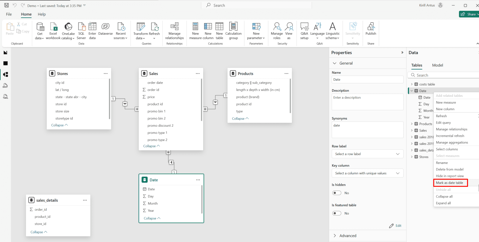
5. Mark a date table as a date table in Power BI.
6. Create data granularity by defining a relationship between two previously unrelated tables: the Date table and the Cost table.
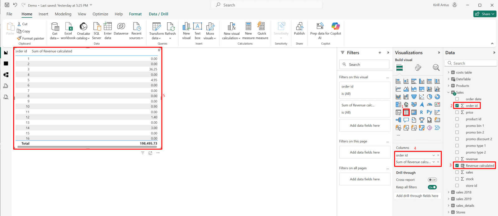
7. Create model calculations using DAX measures and calculated columns.
8. Create calculations using the CALCULATE function in Power BI (DAX).
9. Create a Year-to-Date (YTD) revenue calculation using Time Intelligence in Power BI.
10. Optimize model performance by using the Performance Analyzer.
*
All files used in this project are located here
Important: For this exercise, you need to load the All_cleaned_tables.pbix file.
Note: It is recommended to keep the .pbix file and all CSV files in the same folder, although this is not a strict requirement.
*
Steps
*
Create relationships between tables in the data model (Model view).
Load and clean the data.
1. Load the dim_products and dim_stores tables into Power Query.
Click on "Get data" → Text/CSV → Connect

*
Click "Transform Data" to open the data in the Query Editor.

*
2. Load the dim_stores tables into Power Query.
From Power Query, click "New source" → Text/CSV, then OK

*
3. In the dim_products and dim_stores tables, perform data cleaning.
- In both tables, select Use First Row as Headers.
- Replace underscore with space (in columns name)

*
4. The "store size" column should contain only numbers. Remove any text (like the word "qm") from the column so that changing the data type will not produce an error.
- Select the "store size" column and choose replace values.
- In the "Value to Find" field, enter a space followed by the word 'qm.'
- Leave the Replace with field empty.
Note: This will delete everything after the space, including the word 'qm.'

*
5. Change the data type to a whole number.
- Right-click on "store size" column → Change type → Whole number

*
6. Rename dim_stores to Stores and dim_products to Products.

*
Create relationships between tables.
1. Make sure the "Auto detect relationship after data is loaded" feature is enabled.
- Go to → File → Options and settings → Options → Data load

*
2. After cleaning and loading the data, the next step is to define relationships between dimension tables (such as Products) and the fact table (such as Sales).
Dimension tables contain descriptive information, while the fact table contains measurable data (e.g., sales).
By creating relationships (usually one-to-many from dimension to fact), Power BI can:
- Filter fact data based on dimension selections.
- Enable accurate reporting and analysis.
- Support proper data modeling using a star schema structure.
Drag & drop the "store id" column from the Sales to the Stores table.

*
3. New relationship window will appear
- Click save

*

*
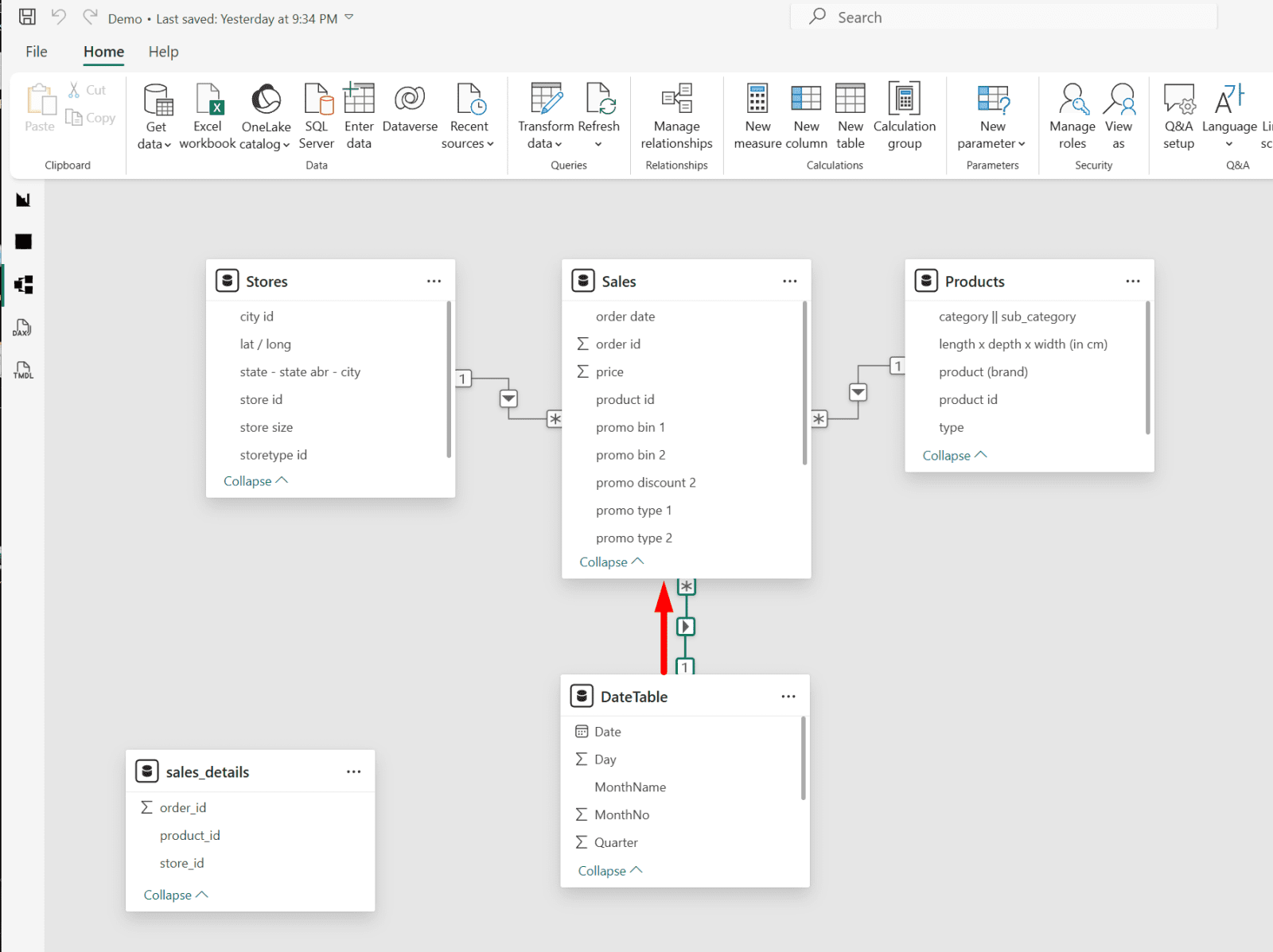
Explained
In the Model view, we see a relationship between the Stores table and the Sales table.
What this relationship shows:
- The Stores table is a dimension table.
- The Sales table is a fact table.
- The relationship is created using the store_id column.
It is a *many-to-one (1 : ) relationship:
- 1 on the store's side
- * (many) on the Sales side
- One store can have many sales records.
- But each sale record belongs to only one store.
What this means:
- Each store_id appears once in the Stores table.
- The same store_id can appear many times in the Sales table.
- One store can have many sales records.
Filter Direction:
- The arrow in the relationship indicates the filter flow direction:
- When you select a store (for example, in a slicer),
- Power BI filters the related sales records automatically.
Why this is important:
This relationship allows:
- Accurate aggregation of revenue, sales, and stock per store.
- Filtering reports by store, state, or city.
- Proper implementation of a star schema model.
*
4. Drag and drop "product id" from Products to Sales table → Click Save

*
What will happen:
A relationship will be created between:
- Products (product_id)
- Sales (product_id)
It will be a *one-to-many (1 : ) relationship:
- 1 on the Products side (each product appears once)
- * on the Sales side (a product can appear many times in sales)
- In short, one product can have many sales
The default cross-filter direction will usually be
- Single direction (from Products → Sales)

*

Cross filter direction in Power BI
Single → Filters flow one way only.
- Example: From Products → Sales.
- If you filter a product type, it will filter sales, but filtering sales doesn’t filter products.
Both → Filters flow both ways.
- Example: From Products ↔ Sales.
- Filtering products filters sales, and filtering sales filters products.
Useful for many-to-many relationships or when you want visuals to interact freely in both directions.
Note: Use both carefully, it can slow down your model if you have large tables.