Preparing data for analysis is a critical first step in any data project. It ensures that the data is clean, consistent, and structured in a way that makes analysis accurate and efficient. This process involves connecting to data sources, transforming and shaping tables, handling inconsistencies, and applying best practices for data organization..

This guide is designed to be followed in sequence:
Part 1 - Advanced Data Preparation in Power BI
Part 2 - Model the Data with power BI
Part 3 - Visualization and Report Creation with Power BI
Part 4 - Power BI Report Deployment & Management
*
Task Details
1. Establish a connection to a CSV data source.
2. Change the file path in the source settings if the file is moved to a different location.
3. Shape and transform tables by removing rows and columns and promoting the first row to a header.
4. User-friendly naming convention.
5. Resolve inconsistencies and handle null values by replacing values and removing duplicates.
6. Evaluate and transform the data types of columns.
7. Learn how to append and merge queries, pivot and unpivot columns, and add conditional columns to prepare data for analysis.
8. Perform data profiling to identify potential problems in the data and resolve errors.
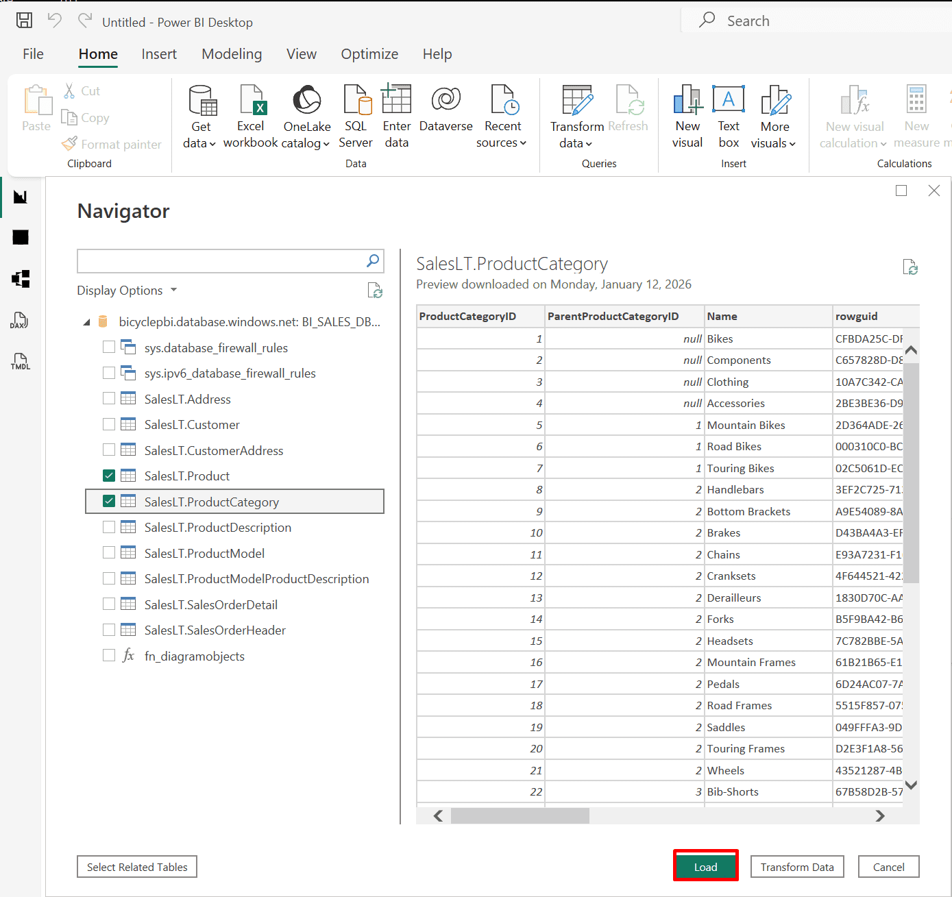
9. Importing Data from Folders and Azure SQL Database (Import or DirectQuery)
*
All files used in this project are located here
Steps
Establish a connection to a CSV data source.
Connect to CSV file
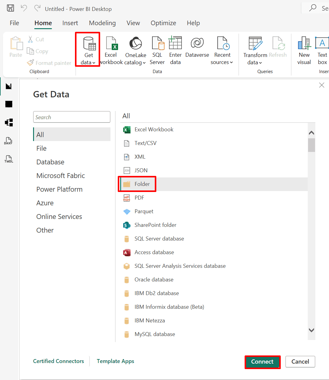
1. In Power BI Desktop go to Home tab then click on "Get data."

*
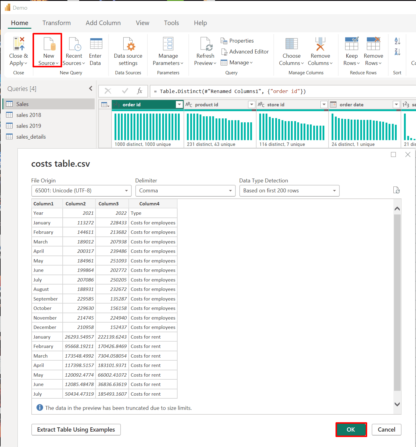
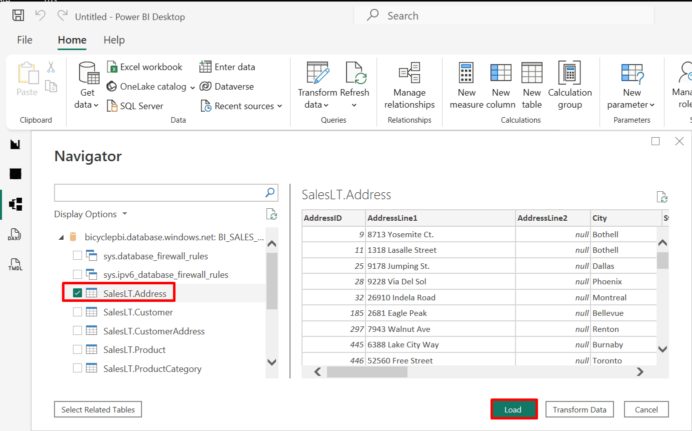
2. Select your CSV file.
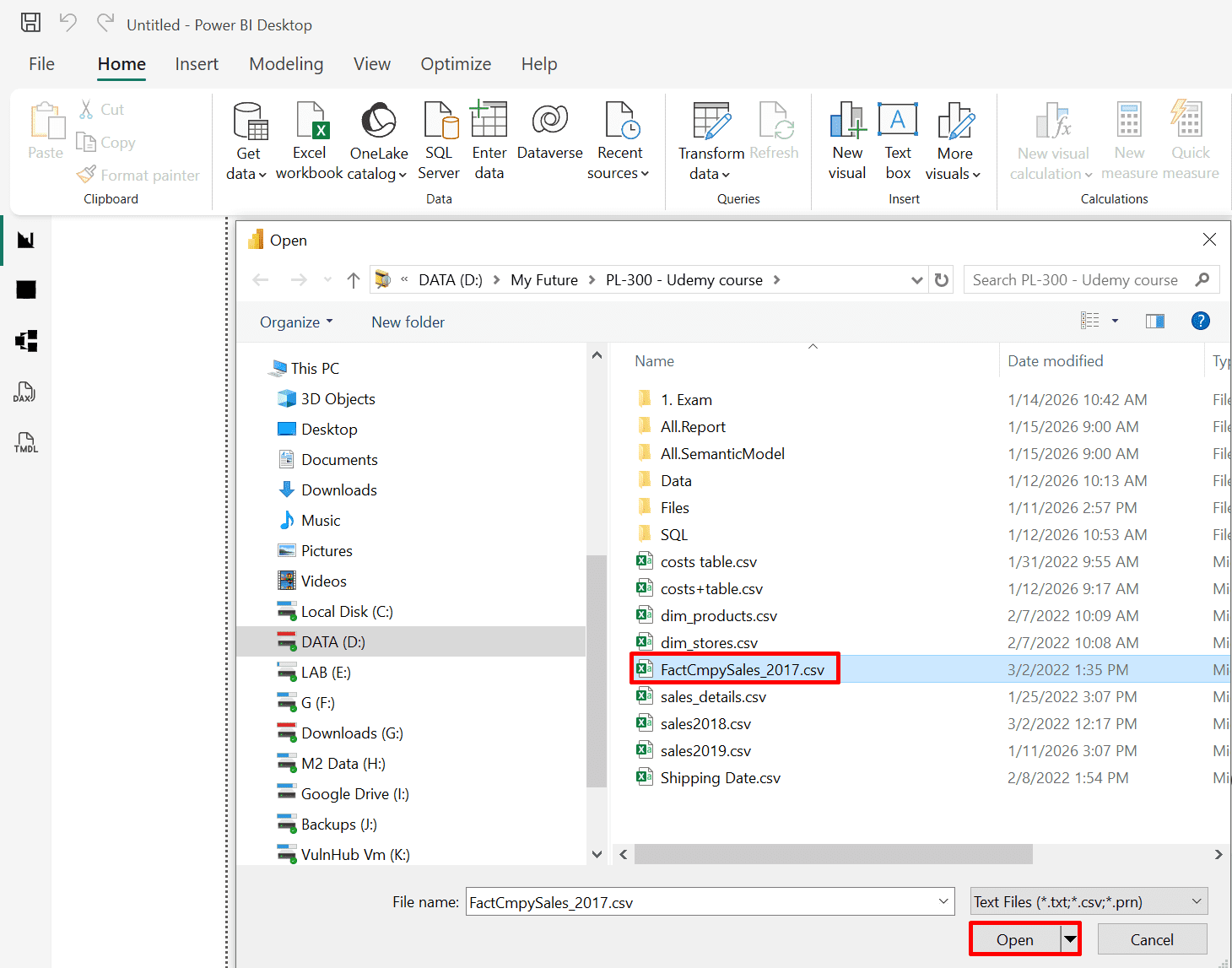
*
3. Click "load" to load the CSV file.
Note: You could also click the "Transform Data" button to clean and transform the data automatically.
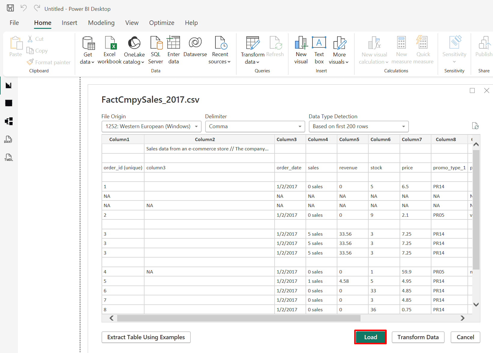
*
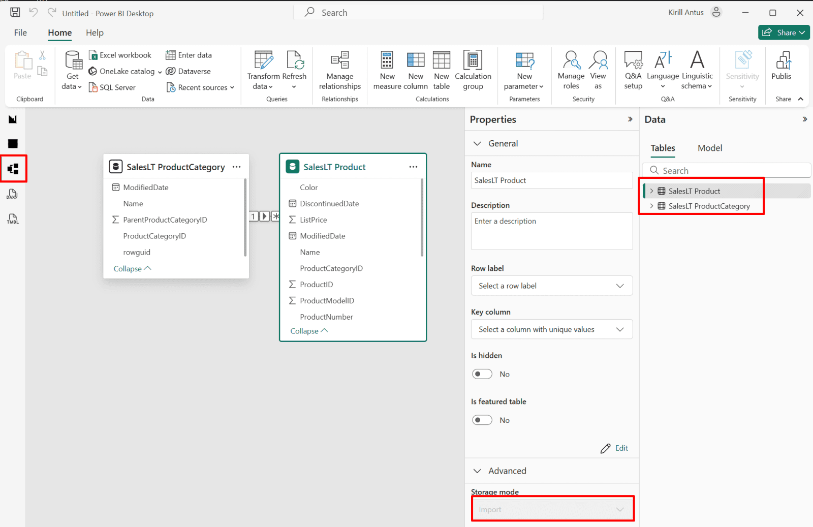
4. You can see the loaded file on the right side.
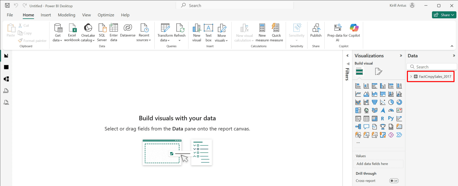
*
Change the file path in the source settings if the file is moved to a different location.
1. In case you move the file to a different location, you will have to change the file path as follows:
Go to "Transform data" and choose "Data source settings."
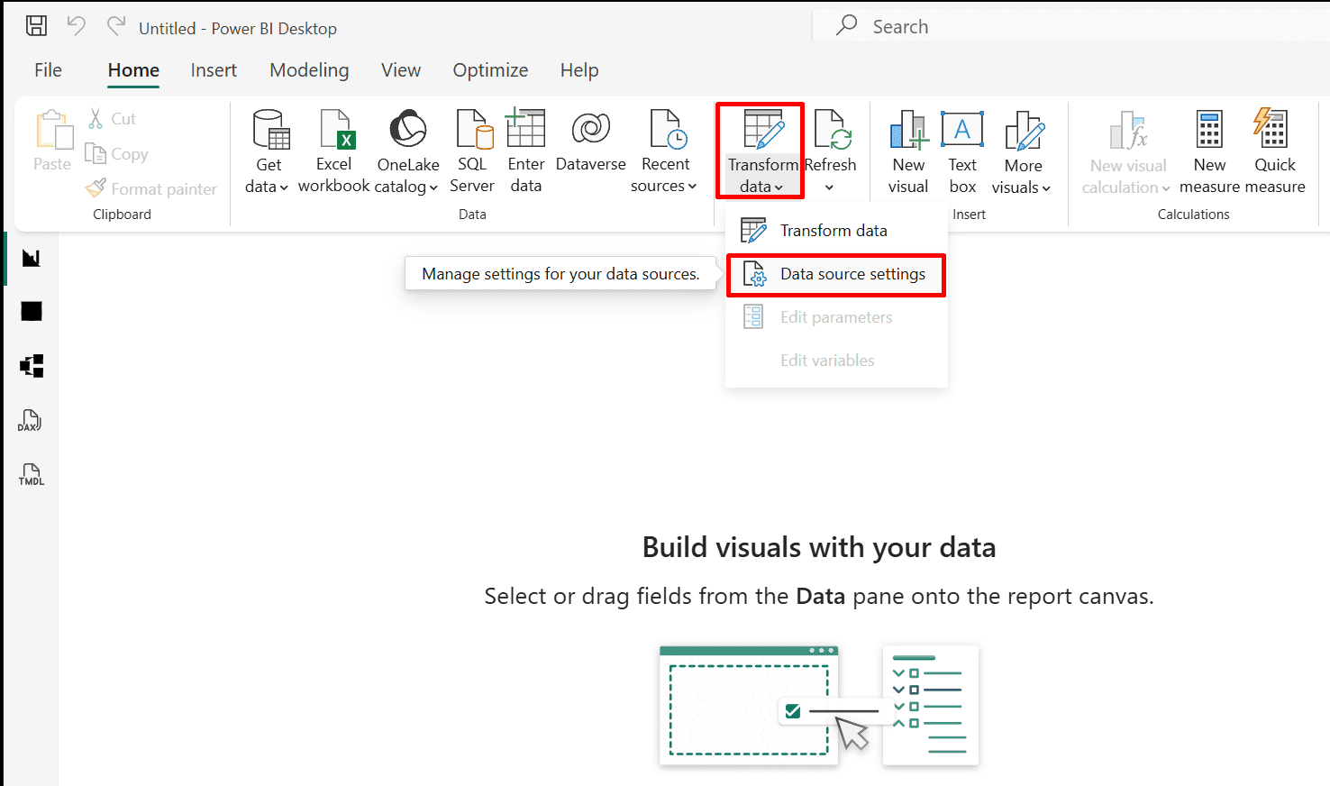
*
2. Click the "Change source..." and choose new file location.

*
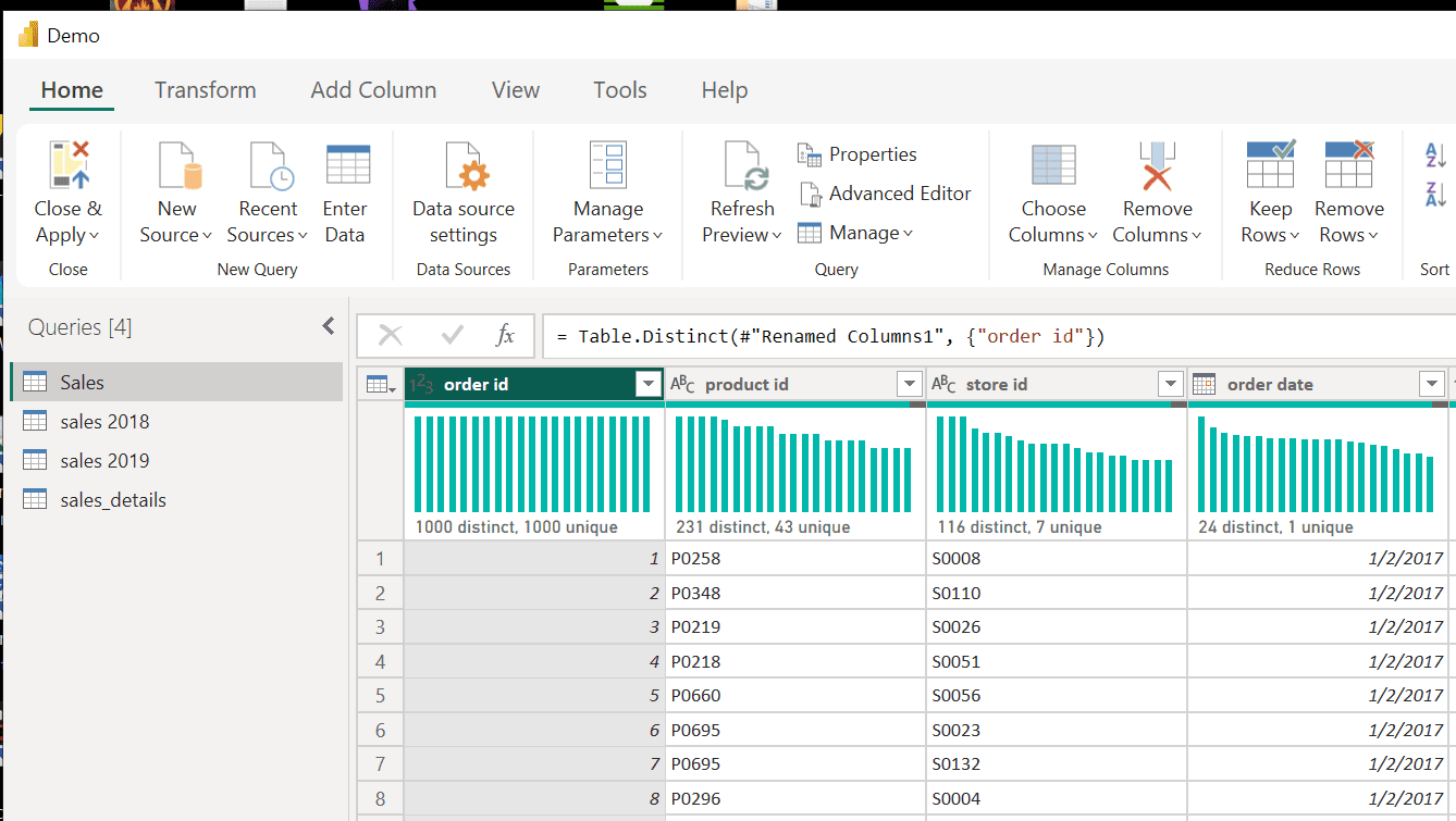
Shape and transform tables by removing rows and columns and promoting the first row to a header.
1. Click on "Transform data" to enter the Power Query editor.
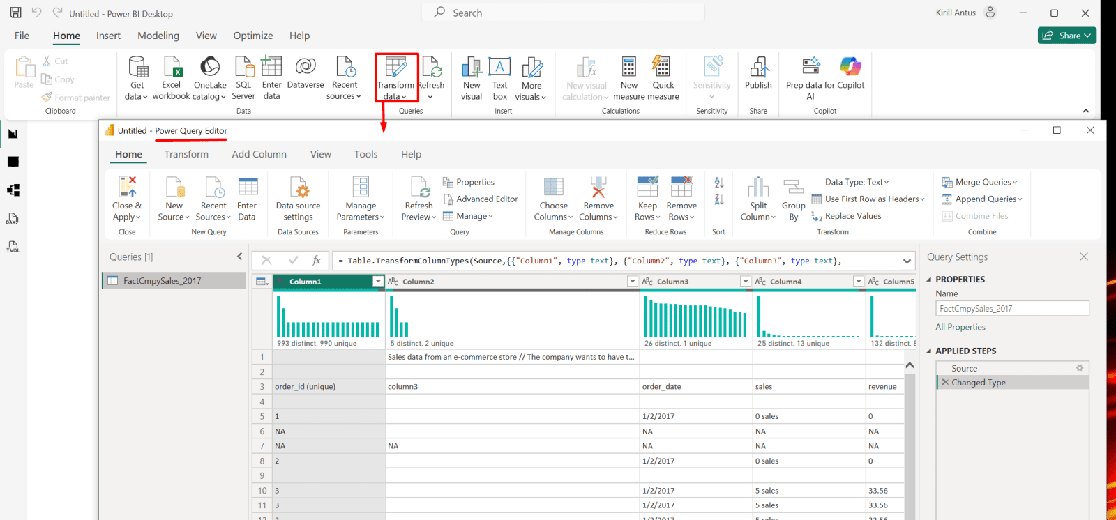
*
2. Delete the first two rows and use the third row as a column header.
Select the third row and click on "Remove rows" then "Remove top rows."

*
3. Specify how many rows to remove, then click OK.

*
4. Promote the first row as a column header.
Note: Use the same method to remove the first blank row.

*

*
5. Remove Column 3 because it is empty.
Right-click on the column and choose remove.

*
6. To apply your changes, click Apply or Close & Apply if you are done modifying the data.

*
7. You can see that the changes took effect on the right side.
Note: To return to Power Query, click Transform Data.